Summary
Idaho Irrigation District and New Sweden Irrigation District (Districts) are promoting the County Line Hydroelectric Project (CLHP), which will divert water from about 3.5 miles of the Snake River north of Idaho Falls for hydroelectric plant feed. Hydroelectric discharge will be returned to the Snake River. The portion of the Snake River affect by the water diversion is known as the Osgood Reach.
Districts are requested that the Federal Energy Regulatory Commission (FERC) issue a license to allow them to divert water around the Osgood Reach provided they maintain a 1,000 cfs (cubic feet per second) minimum reach bypass flow (MBF). The term “bypass” refers to water they stays in the river and bypasses the hydroelectric plants.
Historical average winter reach flow (defined as average from October through March) is 2,800 cfs. Reach flow of 1,000 cfs has historically occurred less than 1% of the time. Districts intend to lower reach flow to 1,000 cfs for 30% of the time (more than 30 times more than current) on the average and as long as 6 consecutive months through the winter (more than 50 times more than current).
At issue is whether lowering winter flow from the current average 2,800 cfs to 1,000 cfs will kill trout in the Osgood Reach. Districts submitted a Draft License Application (DLA) to FERC in which they assert that 1,000 cfs is “protective” of the fishery. Districts never actually say in the DLA why 1,000 cfs is more or less “protective” than other possible MBFs. Districts provided results of their habitat preference models (HPM) for various species (rainbow and brown trout) and life-cycles (juvenile and adult) in the DLA; presumably in support of their assertion that 1,000 cfs is “protective” of the fishery.
Habitat Preference (Suitability) Model (HPM)- Description
A habitat preference model uses a computer to divide the reach into numerous individual evaluation elements (for example; 1-meter grids), apply a common set of rules to score each element with regard to habitat suitability, then add scores of all elements.
HPM typically consists of the following:
- Use a computer program (Geographical Information System “GIS”) to cut the river into hundreds of evaluation elements
- Use established models to generate river physical properties for each evaluation element in the affected area (such as water velocity, depth and temperature)
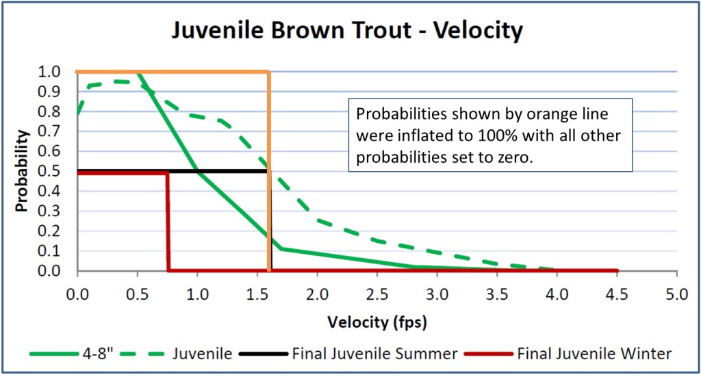
- Use established habitat suitability curves (HSCs) that show probability that habitat will be suitable at prescribed values of river physical properties (example: per the HSCs graphs shown below, a velocity of about 1.6 feet per second gives a suitability probability of 0.5)
- Determine the suitability probability corresponding to each physical property for each GIS evaluation element (Districts used depth, velocity and bottom substrate)
- Combine suitability probabilities for each evaluation element to determine its overall suitability value
- Add suitability values for all elements to produce the suitability value for the entire Osgood Reach at the given river flow rate
- Repeat the above for multiple river flows
- Compare overall suitability values to determine which flow provides the highest suitability
The Districts HPM used a pass/fail approach for suitability…the element was either suitable or it was not. The GIS provided the total area of all suitable elements for a given flow.
Districts’ HPM output consists of area of “usable” habitat as a function of flow for each of three species/life-cycle categories (juvenile, adult rainbow and adult brown trout). FERC’s and Districts’ own staff said that Districts’ HPM ouput regarding area of “usable” habitat as a function of flow is not a proxy for fish overwinter survival as a function of flow; however, Districts appear to be providing HPM results to FERC to support their claim that 1,000 cfs MBF is “protective” of the fishery.
Stakeholders have repeatedly commented that Districts’ use of the term “usable habitat” is misleading because it conveys the false impression that their model results pertain to all potentially usable reach habitat when this is not the case. Districts’ modeled only “best” habitat while not reporting value of all available habitat.
Districts tried to use results of summer HPMs for winter habitat assessment. Summer HPMs combine HSC collected for small streams during the summer with physical properties from flow with no ice. Stakeholder (state and federal agencies, non-governmental organizations and citizens) overwhelmingly rejected this gross oversimplification and demanded that Districts address impacts of fish behavior during icing conditions. Districts agreed to create winter HPMs.
Districts’ HPM results are useless for FERC project licensing
The Snake River starts at the confluence of the South Fork of the Snake River and the Henry’s Fork of the Snake River. The Osgood Reach is located about 20 miles downstream of the confluence. The South Fork provides about 80% of flow to the Snake River.
Districts successfully argued to Stakeholders and the FERC that juvenile rainbow and brown trout habitat should be modeled identically.The figure below contains Districts’ winter juvenile HPM results overlaid on decades of Idaho Department of Fish and Game (IDFG) empirical data regarding overwinter juvenile trout survival in the South Fork Snake River as function of winter flow. IDFG data for the South Fork is applicable to the Osgood Reach because the South Fork is the same river located in the same geographic region and climatic region with similar flow. Each open black circle in the figure represents one year of IDFG empirical data.
IDFG empirical data shows that lowering winter flow below 3,000 cfs will kill juvenile trout. Districts’ HPM results for juvenile trout shows that more area of usable habitat is available as reach flow declines, which Districts imply means that lower flows are better for overwinter survival of juvenile trout.
Computer models are validated by whether model results match empirical (measured) data. Districts’ winter juvenile trout HPM results are either: 1) invalid because they predicts results opposite of IDFG empirical data or 2) are such a poor indicator of overwinter survival that they are useless for this purpose.
Separate HPMs are completed for various bypass flows for different species (rainbow and brow trout) and life-cycle (juvenile or adult). It is reasonable to suspect that all Districts winter HPM results as useless as their juvenile trout model because Districts used the same flawed methodology for all their winter species/life-cycle HPMs.
Districts assertion that a 1,000 cfs MBF is “protective” of juvenile trout is directly refuted by decades of empirical data collected by the Idaho Department of Fish and Game (IDFG) as well as other standard metrics for determine protective flow. All of the following are consistent regarding minimum flow to protect the fishery:
- 3,000 cfs minimum protective flow per IDFG empirical data for juvenile trout on the South Fork
- 2,880 cfs minimum protective flow per the Tennant method (link to website tab: Tennant Method)
- 2,800 cfs to 4,100 cfs minimum protective flow per the wetted area method (link to website tab: USGS Wetted-Perimeter Method);
- Many of Districts’ literature references state that lower flow in the winter or early spring kills trout
- Districts could not find one literature reference world-wide that stated lower flow during the winter enhance trout overwinter survival.
Districts’ invalid winter juvenile HPM results are an extreme outlier to all other data available to inform the FERC regarding appropriate MBF to protect the fishery.
Deficiencies in Districts Winter HPMs
The relevant point is that the Districts’ winter HPM results are useless for purpose of estimating trout overwinter survival as a function of flow. The reason they are useless is academic.
Districts winter HPMs suffer from the classic cliche of computer modeling, which is “garbage in = garbage out”. Districts HPMs have numerical biases that skew results to show more suitable habitat at lower flows, but fundamentally suffer from that there is no credible winter habitat suitability criteria and it is essentially impossible to generate credible river physical property data when ice is present.
Districts’ HPMs suffer from the following fatal flaws:
- Districts’ primary literature reference (Huusko et al.) states that little information exists regarding overwinter salmonid survival in large rivers and even basic generalized winter habitat preference curves (based on small streams) used in habitat-hydraulic modelling are almost totally lacking for young salmonids (trout) in winter
- Districts cite multiple references stating that a positive correlation exists between increased winter and spring flows and overwinter trout survival. Districts could find not a single reference world-wide that states reducing winter flow enhances overwinter trout survival.
- Districts state in their icing study plan: “No known quantitative methods exist for comprehensive prediction of ice formation and its effect on aquatic resources.” FERC staff, federal and state agency staffs, stakeholders and the Districts all commented during a January 21, 2016 meeting that ice modeling is complex and no generally accepted method exists to determine river ice formation.Districts offer “opinions” regarding ice formation as a function of flow (and therefore prediction of river physical properties) in lieu of quantitative modeling of river physical properties as a function of flow.
- Districts state in their final icing study: “There are no specific equations for the development of anchor ice, shore ice, or its growth.” Winter river physical properties as a function of flow were developed by the Districts assuming ice formation mechanisms are essentially the same over a very wide range of flows.
- Districts state in the study plan without justification: “The modeling would be performed for the ‘peak ice’ condition only, representing the maximum impact to fish and wildlife habitat during the ice season.” Peak ice is a relatively rare circumstance during which ice that otherwise exists to the river bottom is lifted with the area underneath deemed eligible for suitable habitat designation because it becomes wetted. Partial ice cover conditions exist during most of the time that ice is present. During partial ice cover conditions, habitat deemed suitable at many locations subject to “peak ice” conditions would be unsuitable because the water column would be frozen to the river bottom. Considering area of ice to the river bottom, partial ice cover would more likely result in maximum impact to fish than would peak icing conditions.
- Districts winter habitat suitability criteria (HSC) curves have no basis in literature. Districts admit that at the time the original HSC were established, it was recognized that the winter HSC lacked established curves to use as reference. Districts winter HSC curves for the large Snake River during winter are guesses based on adjusting summer HSC developed for much small streams.
- Districts collected no HSC data during icing conditions. “Winter” HSC was collected at temperatures between 40 and 50 degrees F with no ice present.
- Fishery professionals that prepared winter HSC have no prior experience in development of winter HSC.
- Fishery professionals that prepared winter HSC don’t agree whether water column average velocity or minimum velocity should be applied to HSC.
- Districts substituted summer HSC data developed for small streams for winter HSC data for much larger rivers with no statistical justification; a practice not supported by Districts’ most prominent reference (Huusko et al.).
- Districts used a single set of HSC curves over a wide range of flows even though their cited reference Armstrong et al 2003 states: “Recent work has shown that the method can be misleading when applied to Atlantic salmon and brown trout because preference curves are sensitive to density (Greenberg, 1994; Bult et al., 1999) and vary with discharge (Holm et al., 2002). New methods are needed to model effects of discharge on fish.” Districts’ use of a single set of HSC curves over a range of flow mathematically biases results to inflate relative area of suitable habitat at lower flows.
- Districts reduced maximum suitable velocity on truncated summer HSC curves to account for that trout are found at lower velocities during winter. This adjustment appears based on the unsupported premise that from summer to winter, a juvenile trout will move to an area of lower mean column velocity instead of simply dropping closer to the bottom at the same location to find a suitable velocity. Districts’ reduction in maximum suitable velocity biases winter juvenile model results to inflate suitable habitat at lower flows.
The FERC must consider that no competent input data exists upon which to base a winter trout habitat model.